Supplementary User's Guide

This version of GAUSSIAN03 has been modified and tested by Prof. Piotr Skurski[1] while working in The Simons Group at The Henry Eyring Center for Theoretical Chemistry.

Introduction

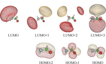
When studying metastable electronic states that can decay by ejection of an electron, one cannot straightforwardly employ variation-based electronic structure tools[2]. For such cases, the lowest-energy state corresponds to that of a free electron (infinitely distant and with zero velocity) plus a system with one fewer electrons. Standard methods thus suffer so-called variational collapse and tend to converge to such "free-electron" descriptions. Let's consider an example offered by the formamide molecule near its equilibrium geometry. The π-symmetry molecular orbitals (MOs) are depicted qualitatively below where their nodal characteristics are emphasized. The lowest two π MOs describe the delocalized π bonding and non-bonding orbitals. The unoccupied MO is the anti-bonding π* orbital.

An SCF calculation using a correlation consistent augmented polarized valence double-zeta (aug-cc-pVDZ) basis set produces the orbitals shown below. The orbital energies for the bonding and non-bonding π MOs (labeled HOMO-2 and HOMO) are -15.4 and -11.5 eV, respectively. The HOMO-1 orbital is a lone pair orbital on the oxygen atom.

The SCF orbital energy of the lowest unoccupied molecular orbital (LUMO) is 0.72 eV, which suggests that an electron of 0.72 eV might attach to produce the formamide anion. However, as the picture shown below illustrates, the LUMO is not even of π* symmetry, nor is the LUMO + 1 or the LUMO + 2 orbital. In fact, these three unoccupied orbitals do not have any significant valence character; most of their amplitude is outside the formamide molecule's molecular skeleton. They are, within the finite atomic orbital basis used, approximations to the free-electron orbital.

The lowest unoccupied orbital of π* character is the LUMO + 3, which is also shown below, and this orbital has an energy of + 2.6 eV. However, in a different atomic orbital basis, the lowest unoccupied orbital of π* symmetry would not necessarily be LUMO + 3, nor would it necessarily have an orbital energy near 2.6 eV.

To give the reader an idea of how these orbitals look for other atomic orbital basis sets, we show below four of the orbitals obtained when a 6-31G** basis is employed.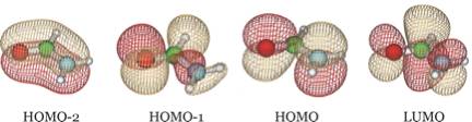

We see that the HOMO-2 and HOMO are still π bonding and non-bonding orbitals and HOMO-1 is still an oxygen lone pair orbital, but now LUMO is the π* anti-bonding orbital. It is important to notice that the desired π* orbital may be the LUMO in one basis but might be another orbital in a different basis as it is in the examples shown above.

Clearly, estimating the vertical electron affinity (EA) by using the energy of the LUMO is wrong, but we need to make clear what is wrong and how to properly identify the correct orbital. In fact, most of the low-energy vacant orbitals are nothing but attempts, within the finite orbital basis used, to represent a free electron plus a neutral formamide molecule. This illustrates the variational collapse problem mentioned above.

Let us now explain how we can fix this error. To focus on the problem, we consider the effective potential that an electron approaching a formamide molecule from afar would experience. Also keep in mind that, as is conventional in electron scattering calculations, we may wish to decompose the wave function describing this "attached" electron into products of radial and angular terms:

(1)

Substituting such an expansion into the Schrödinger equation

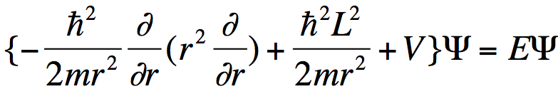. (2)

produces the usual set of coupled-channel equations. Multiplying the Schrödinger equation on the left by Y*_L,M and integrating over the angles θ and ϕ, one obtains a radial equation for the ψ_L,M component of the wave function:

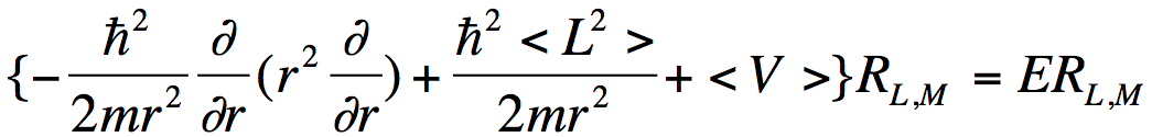. (3)

where <V> denotes the angular average of the electron-molecule potential

. (4)

When the distance r of the electron from the molecule is large, <V> is dominated by an attractive Coulomb factor if the electron is interacting with a cation, by a charge-dipole potential if the electron is interacting with a polar neutral molecule, and by a repulsive Coulomb factor if the electron is interacting with a negative ion. However, the centrifugal potential ћ²<L²>/2mr² always varies as r ^‑2.

For the formamide case at hand, the longest-range component of <V> is the charge-dipole term, which varies as r^-2. Moreover, the nodal character of the π* orbital into which the incoming electron is to attach has dominant L = 3 character. To see this, we view this orbital from a long distance at which its three nuclear centers are nearly on top of one another as shown below.

When viewed as having the O, C, and N nuclei on top of one another, this π* orbital clearly has nodal properties like that of an f-orbital which is why L = 3 is dominant at large-r.

An electron in an orbital having angular momentum L experiences an effective radial potential (i.e., the sum of <V> and the centrifugal potential) that varies as shown qualitatively below for a neutral molecule. For an electron interacting with an anion, the repulsive long-range part of the potential would also include a Coulomb term e²/r. In such cases, the barrier that acts to constrain the electron in the metastable state arises from both Coulomb and centrifugal factors. Nevertheless, the methods discussed here can still be used to characterize the metastable state's energy and wave function.

If, as in the case of formamide, the component of the potential generated by the attractive valence-range influences of the O, C, and N centers is not strong enough, no bound state of the anion will exist[3]. For such a case, only the metastable so-called L = 3 shape resonance state will occur and it will have an energy (the heavy horizontal line) and a radial wave function as shown below.

In the valence region, the resonance function has large amplitude, suggesting that the electron is rather localized, it decays exponentially in the classically forbidden tunneling region, and it has sinusoidal oscillations beyond this region with the local de Broglie wavelength relating to the electron's kinetic energy.

However, at energies both above and below that of the shape resonance state, there exists a continuum of other states. Those lying below the resonance energy vary with r as shown below.

They have little amplitude in the valence region and have large amplitude at large-r and they have longer de Broglie wavelength and thus lower energy than the resonance state. There are also non-resonant states lying energetically above the shape resonance; they have little amplitude in the valence region and larger amplitude at large-r but with shorter de Broglie wavelength corresponding to higher kinetic energy.

So, how can we identify and characterize the resonance wave function (and its energy) when it is "buried" within a continuum of higher- and lower- energy states? The example discussed earlier makes it clear we cannot rely on the orbital energy nor on choosing the LUMO to find the desired state. In the nuclear charge stabilization method[4], we attempt to smoothly slightly enhance the valence-region attractive character of the potential V that the attached electron experiences to an extent that pulls the energy of the metastable resonance state below zero thus rendering it stable[5]. We do this by altering the nuclear charges of those atoms over which the resonance MO is expected to be localized in the valence region. For formamide, we alter the O, C, and N nuclear charges from their actual values of 8, 6, and 7, respectively, to, for example, 8+δq, 6+δq, and 7+δq, respectively. The nuclear charges appear in the electronic Hamiltonian in the electron-nuclear interaction potential

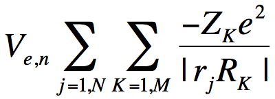. (5)

where the sum over j runs over all N electrons, the sum over K runs over all M nuclei of charge Z_K. So, the nuclear charge scaling in formamide introduces an additional one-electron potential

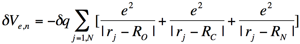(6)

that acts to differentially stabilize the electron's potential energy near these nuclear centers. Visually, we can represent the effects of the scaled nuclear charges on the electron-molecule potential as shown below.

Here, in black, we reproduce the original unscaled potential and its resonance wave function. In blue and red, we illustrate potentials in which the nuclear charges have been incremented by small (blue) or somewhat larger (red) amounts. The key thing to notice that is, if the nuclear charge enhancement is large enough, the valence-range component of the potential will be lowered enough to render the resonance state bound (notice the lack of continuum components at large-r and notice that the energy lies below zero) rather than metastable and thus amenable to studying using conventional variational-based quantum chemistry tools. In this manner, one can carry out conventional calculations on the nuclear charge enhanced species for a series of δq values (all of which must be large enough to render the desired state bound) and then extrapolate to δq→0 to allow the resonance state to be identified from the finite-δq calculations' data.

In practice, to use the nuclear charge stabilization method, one (for a series of δq values)

1. Identifies those nuclei over which the valence component of the desired resonance state's orbital will be distributed;
2. Modifies the nuclear charges of these nuclei (one need not use equal charge increments for all the nuclei[6]) by increasing them by an amount δq;
3. Carries out a standard, bound-state, quantum calculation (SCF, MPn, coupled-cluster, or whatever) on the electron-attached[7]and non-attached states using the scaled nuclear charges to obtain attached (E*) and non-attached (E) state energies, after which
4. One plots the energy difference (E-E*) vs. δq but using only δq values large enough to render E-E* > 0 (i.e., to make the attached state bound relative to the non-attached state), and
5. One then extrapolates the plot to δq→0 to obtain an estimate of the energy of the electron-attached state relative to that of the parent non-attached species (i.e., in the extrapolation, one will find E-E* negative, meaning the electron attached species lies above its parent).

In this manner, one achieves a nuclear charge stabilization estimate of the energy of the desired metastable state.

In the figure shown below, we show Koopmans' theorem[8], SCF-level, MP2-level, and coupled-cluster level energy differences (D) for the formamide and formamide π* anion obtained using the aug-cc-pVDZ  basis set discussed earlier. Only for values of δq equal to 0.18 or larger was the anion found to be electronically stable, so only data obtained with δq = 0.18 and higher were used in constructing these plots.

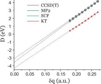
The δq→0 extrapolated energies for each case are as follows:

D = –4.3 eV (KT, red) and the fit's correlation coefficient (squared) is: r² = 0.99957.

D = –3.6 eV (SCF, blue), r² = 0.99996

D = –3.1 eV (MP2, green), r² = 0.99994

D = –3.1 eV (CCSD(T), magenta),  r² = 0.99994.

When analogous nuclear charge stabilization calculations are performed using the 6-31G** basis, the plot shown below results.

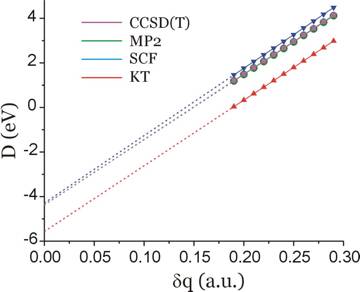
For this basis set, the extrapolated predictions of the D-values are as follows:

D(KT) = -5.6 eV

D(SCF) = -4.3 eV

D(MP2) = -4.4 eV

D(CCSD(T)) = -4.4 eV.

These extrapolations represent the nuclear charge stabilization's predictions for the energy of the anion's metastable π* resonance state relative to that of the neutral for each level of theory.

In addition, below we show the π* LUMO obtained for the aug-cc-pVDZ basis set for δq = 0.19 and 0.26 to show how it differs significantly from the LUMO obtained in the non-scaled calculation which, as we explained earlier, cannot be trusted to relate to the desired resonance state.

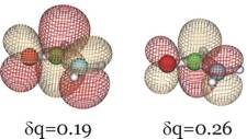
Clearly, this orbital has the desired valence character and nodal pattern. For δq = 0.26 it is more compact than for δq = 0.19 because of the enhanced nuclear attraction in the former case. For the 6-31G** basis, this same orbital is shown below also for δq = 0.16 and δq = 0.29.

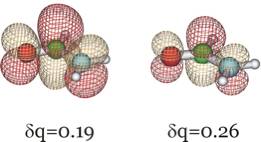
We see that the qualitative character of the desired π* orbital does not depend on the basis set employed although the quantitative values of the resonance state energy do. For the larger basis and using the highest-level of theory (the CCSD(T) data), the π* attached anion is predicted to lie 3.1 eV above the neutral formamide at the neutral's equilibrium geometry. Experiments using so-called electron transmission spectroscopy methods find[9] a resonance state to lie ca. 2 eV above the neutral, so one can see that obtaining accurate estimates of the energies of such metastable states is difficult even when rather good atomic basis sets are employed.

Details for using the G03 modifications

There are two steps that must be taken; one must identify those nuclei whose charges are to be altered and one must tell by how much to increase or decrease the charge of each nucleus.

Specifiying the nuclear centers whose charges are to be modified

IOp(3/110=N_max) and IOp(7/110=N_max)

These IOps are used to tell Gaussian the highest numbered nuclear center range of atoms (centers in the geometry input list in your Gaussian .com file) in which there are the nuclei whose charges are to be modified.

Warning: the largest possible value for this option is 90 in both overlays (see the Limitations and known problems section at the end of this manual), so make sure you number your atoms so that all of the atoms you intend to subject to charge scaling occur within the first 90 atoms.    

Modifying the nuclear charges on the selected centers

IOp(3/111-200) and IOp(7/111-200)

These IOps are used both to denote the centers to be modified and to specify the additional charge (δq) that is to be added to that center (or subtracted from it).

To modify nuclear charge on center #N, the IOptions 3/(110+N) and 7/(110+N) must be set to a proper value.  The additional charge to be added to (or subtracted from) the N^th nucleus must be multiplied by 10⁵ (100000) and set as the value in both IOptions 3/(110+N) and 7/(110+N).

Input examples

Here we present a few examples of Gaussian03 input files showing single-point energy calculations and geometry optimization jobs that involve modified nuclear charges.

%chk=testSP
#p RHF 6-31G(d) SCF=(Tight,NoVarAcc,Maxcycle=512,IntRep)
   GFInput IOp(6/7=3) IOp(3/32=1)
   IOp(3/110=3,3/111=33000,3/112=34000,3/113=33000)
   IOp(7/110=3,7/111=33000,7/112=34000,7/113=33000)

Test job #1

0  1
 O
 C  1 co2
 N  2 nc3        1 nco3
 H  2 hc4        1 hco4         3 dih4
 H  3 hn5        2 hnc5         1 dih5
 H  3 hn6        2 hnc6         1 dih6

co2         1.277811
nc3         1.496812
nco3        116.154
hc4         1.002000
hco4        135.119
dih4        172.107
hn5         1.004634
hnc5        107.935
dih5       -119.695
hn6         1.002000
hnc6        112.357
dih6          0.000

%chk=testOPT#p UHF 6-31G(d) SCF=(Tight,NoVarAcc,Maxcycle=512,IntRep)
   GFInput IOp(6/7=3) IOp(3/32=1) OPT GUESS=READ
   IOp(3/110=3,3/111=33000,3/112=34000,3/113=33000)
   IOp(7/110=3,7/111=33000,7/112=34000,7/113=33000)

Test job #2

-1  2
O
C  1 co2
N  2 nc3        1 nco3
H  2 hc4        1 hco4         3 dih4
H  3 hn5        2 hnc5         1 dih5
H  3 hn6        2 hnc6         1 dih6

co2         1.277811
nc3         1.496812
nco3        116.154
hc4         1.002000
hco4        135.119
dih4        172.107
hn5         1.004634
hnc5        107.935
dih5       -119.695
hn6         1.002000
hnc6        112.357
dih6          0.000

%chk=testOPT2
#p UHF aug-cc-pVDZ SCF=(Tight,NoVarAcc,Maxcycle=512)
   GFInput IOp(6/7=3) IOp(3/32=1) OPT GUESS=READ
   IOp(3/110=5,3/111=33000,3/112=34000,3/115=33000)
   IOp(7/110=5,7/111=33000,7/112=34000,7/115=33000)

Test job #3

-1  2
O  0.000000    0.000000    0.000000
C  0.000000    0.000000    1.277811
H -0.700350    0.097094    1.987802
H  1.412538   -0.830293    2.498962
N  1.343557    0.000000    1.937584
H  2.094138    0.000000    1.273783

Some limitations and known problems

• The maximum number of centers whose charges can be modified in one job is limited to 90, which is limited by the array size used for storing the IOps.
• The maximum number of atoms in a molecule is not limited other than being subject to the same limitations as in any regular Gaussian03 input files.
• The highest possible number for a modified center is 90. This means that the centers must be numbered so that all those to be charge-modified occur in the first 90.
• The modified version of Gaussian03 has been tested for single-point energy and geometry optimization jobs. Calculating harmonic vibrational frequencies is also possible. Note that changing the nuclear charges does not affect the atomic masses, so quantities that depend on atomic masses (such as vibrational frequencies) are calculated in a standard G03 manner.
• The value of the nuclear-nuclear repulsion energy, as well as its contributions to the gradients and Hessians, are calculated using the conventional  (non-modified) nuclear charges.
• Some modifications of the nuclear charges are to be avoided because they can produce unexpected errors. In particular, changing any nuclear charge by 1 a.u. (or more) leads to problems since, de facto, this changes the chemical identity of the element. In such cases errors reported by MinBas appear (due to the comparison made by Gaussian03 in which the atomic number is compared with its nuclear charge).
• In some cases, both the SCF procedure and the geometry optimization process can be more difficult to converge when modified nuclear charges are used, so it is recommended that one use the MaxCycle keyword to increase the number of maximum SCF iterations and optimization steps to improve chances for successful convergence.
• Molecular properties such as populations (e.g., Mulliken population analysis, ESP-fitted charges according to the Merz-Singh-Kollman scheme, etc.), multipole moments, polarizability tensors, and other quantities that depend on the nuclear charges are evaluated with the modified nuclear charges.

Please report any problems to Piotr Skurski.

[1] Chemistry Department, University of Gdansk, Gdansk, Poland

[2] Even methods such as Møller-Plesset perturbation theory (MP) and coupled-cluster theory (CC) suffer from this problem because they are based on a Hartree-Fock (HF) self-consistent field (SCF) initial starting point that is intrinsically variation-based.

[3] For example, the ²Π state of NO is electronically stable relative to NO⁺ plus an electron , but the ²Π state of the isoelectronic species N₂^- is metastable. The increased electronegativity of the oxygen atom in NO compared to that of the nitrogen atom in N₂^- is enough to make the valence-range potential attractive enough to make NO stable.

[4] This method was introduced by the Peyerimhoff group (see, for example, B. Nestmann and S. D. Peyerimhoff, J. Phys. B. 18, 615-626 (1985); J. Phys. B 18, 4309-4319 (1985)) and is based on the stabilization theory put forth by Howard Taylor (see, for example, Taylor, H. S. Adv. Chem. Phys. 1970, 18, 91).

[5] Alternatively, it is possible to alter the large-r character of the wave function by either placing the system inside a large spherical "box" of radius R. By then varying the radius R, one can vary the de Broglie wave lengths of the orbitals generated. This, in turn, would allow one to ultimately identify a box size R that, within the finite orbital basis set employed, can generate an orbital (not necessarily and probably not the LUMO) that has a large valence-range component and a large-r component whose de Broglie wave length (and thus energy) is appropriate. The variation of the 'box' radius R can, in practice, be achieved by scaling the orbital exponents of the more diffuse basis functions (larger orbital exponents represent a smaller box). However, we have found this procedure to be more cumbersome than that which we have decided to automate in making our changes to G03.

[6] That is, one can use a different value δq_K for the K^th nucleus, but we have found it sufficient to increase the nuclear charges of all the nuclei over which the resonance orbital extends by equal amounts. Because one obtains the prediction of the resonance state's energy by extrapolating to δq→0, it should not matter much whether one uses the same or different values of δq for the different nuclei.

[7] In carrying out the SCF calculations (that also form the starting points of the MP2 and CCSD(T) calculations), one must be careful to singly-occupy the desired orbital (i.e., the π* orbital in the formamide case). The increased nuclear charges will act to lower the energy of not only the π* orbital but also of other orbitals that have significant density on the atomic centers whose charges have been enhanced. Thus, one may find that the energy ordering of the virtual orbitals changes as one moves from one δq value to another. As a result, one may need to employ the GUESS=ALTER keyword to maintain single occupancy of the desired orbital as part of the process of generating data to make the energy plots discussed here.

[8] We are defining the Koopmans' theorem electron binding energy to be the negative of the energy of the unoccupied orbital of the neutral molecule rather than the negative of the singly-occupied orbital of the anion.

[9] M. Seydou, A. Modelli, B. Lucas, K. Konate, C. Desfrancois, and J.P. Schermann, Eur. Phys. J. D 35, 199 (2005).